45 multiple data labels excel pie chart

Move data labels - support.microsoft.com Click any data label once to select all of them, or double-click a specific data label you want to move. Right-click the selection > Chart Elements > Data Labels arrow, and select the placement option you want. Different options are available for different chart types. For example, you can place data labels outside of the data points in a pie ... Edit titles or data labels in a chart - support.microsoft.com The first click selects the data labels for the whole data series, and the second click selects the individual data label. Right-click the data label, and then click Format Data Label or Format Data Labels. Click Label Options if it's not selected, and then select the Reset Label Text check box. Top of Page

Create a multi-level category chart in Excel - ExtendOffice 1. Firstly, arrange your data which you will create a multi-level category chart based on as follows. 1.1) In the first column, please type in the main category names; 1.2) In the second column, type in the subcategory names; 1.3) In the third column, type in each data for the subcategories. 2.

Multiple data labels excel pie chart

Add or remove data labels in a chart - support.microsoft.com Click the data series or chart. To label one data point, after clicking the series, click that data point. In the upper right corner, next to the chart, click Add Chart Element > Data Labels. To change the location, click the arrow, and choose an option. If you want to show your data label inside a text bubble shape, click Data Callout. Pie Chart in Excel - Inserting, Formatting, Filters, Data Labels Right click on the Data Labels on the chart. Click on Format Data Labels option. Consequently, this will open up the Format Data Labels pane on the right of the excel worksheet. Mark the Category Name, Percentage and Legend Key. Also mark the labels position at Outside End. This is how the chark looks. Formatting the Chart Background, Chart Styles Select all Data Labels at once - Microsoft Community AFAIK it has never been possible to select all data labels (if there are multiple series) You might be able to use code like this. Sub DL () Dim ocht As Chart. Dim ser As Series. Dim opt As Point. Dim s As Long. Dim p As Long. Set ocht = ActiveWindow.Selection.ShapeRange (1).Chart.

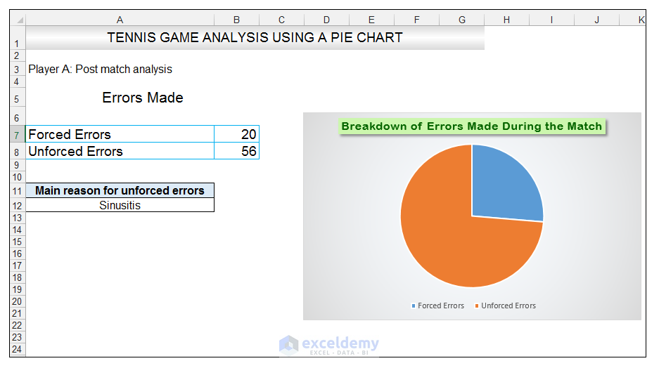
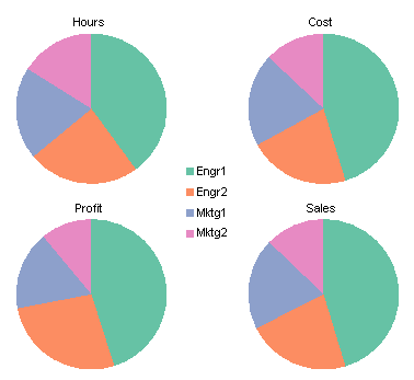
Multiple data labels excel pie chart. How to Make a Multi-Level Pie Chart in Excel (with Easy Steps) - ExcelDemy Step 5: Add Data Labels and Format Them. Adding data labels can help us analyze the information precisely. Right-click on the outermost level on the chart and then right-click on the chart. Then from the context menu, click on the Add Data Labels. After clicking on the Add Data Labels, the data labels will show accordingly. How to Combine or Group Pie Charts in Microsoft Excel Click on the first chart and then hold the Ctrl key as you click on each of the other charts to select them all. Click Format > Group > Group. All pie charts are now combined as one figure. They will move and resize as one image. Choose Different Charts to View your Data How to Make a Pie Chart with Multiple Data in Excel (2 Ways) - ExcelDemy In Pie Chart, we can also format the Data Labels with some easy steps. These are given below. Steps: First, to add Data Labels, click on the Plus sign as marked in the following picture. After that, check the box of Data Labels. At this stage, you will be able to see that all of your data has labels now. Show multiple data lables on a chart - Power BI For example, I'd like to include both the total and the percent on pie chart. Or instead of having a separate legend include the series name along with the % in a pie chart. I know they can be viewed as tool tips, but this is not sufficient for my needs. Many of my charts are copied to presentations and this added data is necessary for the end ...

Everything You Need to Know About Pie Chart in Excel - SpreadsheetWeb How to Make a Pie Chart in Excel. Start with selecting your data in Excel. If you include data labels in your selection, Excel will automatically assign them to each column and generate the chart. Go to the INSERT tab in the Ribbon and click on the Pie Chart icon to see the pie chart types. Click on the desired chart to insert. Pie Chart in Excel | How to Create Pie Chart - EDUCBA Go to the Insert tab and click on a PIE. Step 2: once you click on a 2-D Pie chart, it will insert the blank chart as shown in the below image. Step 3: Right-click on the chart and choose Select Data. Step 4: once you click on Select Data, it will open the below box. Step 5: Now click on the Add button. Multiple data labels (in separate locations on chart) Re: Multiple data labels (in separate locations on chart) You can do it in a single chart. Create the chart so it has 2 columns of data. At first only the 1 column of data will be displayed. Move that series to the secondary axis. You can now apply different data labels to each series. Attached Files 819208.xlsx‎ (13.8 KB, 265 views) Download Multiple Data Labels on a Pie Chart | MrExcel Message Board Hello All, So I have a table with 8 rows and 3 columns. This table includes: Column 1 - shipment name. Column 2 - shipment cost. Column 3 - shipment weight. I have created a pie chart from this table, which covers the first two columns. Displayed next to each slice is a label with the shipment name, shipment cost, and percent share of the pie.

Formatting data labels and printing pie charts on Excel for Mac 2019 ... 2. When formatting data labels on an extended bar of pie chart: Excel does not allow me to: i format all the data labels at once to show 3 elements: category name, value and percentage. In the label options, I can tick these 3 elements, but chart wont show them. I have to go in and edit each data label in turn. As there are 48, this is not practical. How to group (two-level) axis labels in a chart in Excel? - ExtendOffice You can do as follows: 1. Create a Pivot Chart with selecting the source data, and: (1) In Excel 2007 and 2010, clicking the PivotTable > PivotChart in the Tables group on the Insert Tab; (2) In Excel 2013, clicking the Pivot Chart > Pivot Chart in the Charts group on the Insert tab. 2. In the opening dialog box, check the Existing worksheet ... How to display leader lines in pie chart in Excel? - ExtendOffice To display leader lines in pie chart, you just need to check an option then drag the labels out. 1. Click at the chart, and right click to select Format Data Labels from context menu. 2. In the popping Format Data Labels dialog/pane, check Show Leader Lines in the Label Options section. See screenshot: How to add data labels from different column in an Excel chart? This method will guide you to manually add a data label from a cell of different column at a time in an Excel chart. 1. Right click the data series in the chart, and select Add Data Labels > Add Data Labels from the context menu to add data labels. 2. Click any data label to select all data labels, and then click the specified data label to select it only in the chart.

How to Make a Pie Chart in Excel & Add Rich Data Labels to The Chart!

How to Make a Pie Chart in Excel (Only Guide You Need) From there select Charts and press on to Pie. You can also insert the pie chart directly from the insert option on top of the excel worksheet. Before inserting make sure to select the data you want to analyze. After this, you will see a pie chart is formed in your worksheet.

How to Create Multi-Category Chart in Excel - Excel Board

Creating Pie Chart and Adding/Formatting Data Labels (Excel) Creating Pie Chart and Adding/Formatting Data Labels (Excel) Creating Pie Chart and Adding/Formatting Data Labels (Excel)

How to Make a Pie Chart in Excel Using Spreadsheet Data

Pie Charts in Excel - How to Make with Step by Step Examples Step 3: Right-click the pie chart and expand the "add data labels" option. Next, choose "add data labels" again, as shown in the following image. Step 4: The data labels are added to the chart, as shown in the following image. With these labels, the sales quantity of each flavor is displayed on the respective slice.

How to Make a Pie Chart in Excel & Add Rich Data Labels to The Chart!

How to Create and Format a Pie Chart in Excel - Lifewire Select the plot area of the pie chart. Select a slice of the pie chart to surround the slice with small blue highlight dots. Drag the slice away from the pie chart to explode it. To reposition a data label, select the data label to select all data labels. Select the data label you want to move and drag it to the desired location.

How to Make Charts and Graphs in Excel | Smartsheet

How to add or move data labels in Excel chart? - ExtendOffice In Excel 2013 or 2016. 1. Click the chart to show the Chart Elements button . 2. Then click the Chart Elements, and check Data Labels, then you can click the arrow to choose an option about the data labels in the sub menu. See screenshot: In Excel 2010 or 2007. 1. click on the chart to show the Layout tab in the Chart Tools group. See ...

How to Make a Pie Chart in Excel & Add Rich Data Labels to The Chart!

How to Create Multi-Category Charts in Excel? - GeeksforGeeks Implementation : Step 1: Insert the data into the cells in Excel. Now select all the data by dragging and then go to "Insert" and select "Insert Column or Bar Chart". A pop-down menu having 2-D and 3-D bars will occur and select "vertical bar" from it. Select the cell -> Insert -> Chart Groups -> 2-D Column.

Column Chart to Replace Multiple Pie Charts - Peltier Tech Blog

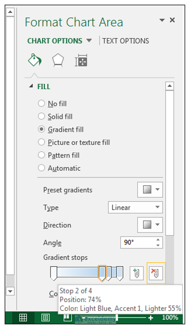
Change the format of data labels in a chart To get there, after adding your data labels, select the data label to format, and then click Chart Elements > Data Labels > More Options. To go to the appropriate area, click one of the four icons ( Fill & Line, Effects, Size & Properties ( Layout & Properties in Outlook or Word), or Label Options) shown here.

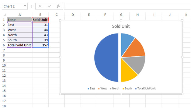
How to Represent Data with a Pie of Pie Chart in Your Excel Worksheet - Data Recovery Blog

Select all Data Labels at once - Microsoft Community AFAIK it has never been possible to select all data labels (if there are multiple series) You might be able to use code like this. Sub DL () Dim ocht As Chart. Dim ser As Series. Dim opt As Point. Dim s As Long. Dim p As Long. Set ocht = ActiveWindow.Selection.ShapeRange (1).Chart.

How to Make a Pie Chart in Microsoft Excel 2010 | Microsoft Excel Tips from Excel Tip .com ...

Pie Chart in Excel - Inserting, Formatting, Filters, Data Labels Right click on the Data Labels on the chart. Click on Format Data Labels option. Consequently, this will open up the Format Data Labels pane on the right of the excel worksheet. Mark the Category Name, Percentage and Legend Key. Also mark the labels position at Outside End. This is how the chark looks. Formatting the Chart Background, Chart Styles