43 how to display data labels in excel

support.microsoft.com › en-us › officeAdd or remove data labels in a chart - support.microsoft.com Right-click the data series or data label to display more data for, and then click Format Data Labels. Click Label Options and under Label Contains , select the Values From Cells checkbox. When the Data Label Range dialog box appears, go back to the spreadsheet and select the range for which you want the cell values to display as data labels. Dynamically Label Excel Chart Series Lines - My Online Training Hub Step 1: Duplicate the Series. The first trick here is that we have 2 series for each region; one for the line and one for the label, as you can see in the table below: Select columns B:J and insert a line chart (do not include column A). To modify the axis so the Year and Month labels are nested; right-click the chart > Select Data > Edit the ...

Custom Data Labels with Colors and Symbols in Excel Charts - [How To ... Step 4: Select the data in column C and hit Ctrl+1 to invoke format cell dialogue box. From left click custom and have your cursor in the type field and follow these steps: Press and Hold ALT key on the keyboard and on the Numpad hit 3 and 0 keys. Let go the ALT key and you will see that upward arrow is inserted.

How to display data labels in excel

Create Dynamic Chart Data Labels with Slicers - Excel Campus 10.02.2016 · Typically a chart will display data labels based on the underlying source data for the chart. In Excel 2013 a new feature called “Value from Cells” was introduced. This feature allows us to specify the a range that we want to use for the labels. Since our data labels will change between a currency ($) and percentage (%) formats, we need a ... How to add text labels on Excel scatter chart axis - Data Cornering Add dummy series to the scatter plot and add data labels. 4. Select recently added labels and press Ctrl + 1 to edit them. Add custom data labels from the column "X axis labels". Use "Values from Cells" like in this other post and remove values related to the actual dummy series. Change the label position below data points. Excel charts: add title, customize chart axis, legend and data labels Click anywhere within your Excel chart, then click the Chart Elements button and check the Axis Titles box. If you want to display the title only for one axis, either horizontal or vertical, click the arrow next to Axis Titles and clear one of the boxes: Click the axis title box on the chart, and type the text.

How to display data labels in excel. Change the format of data labels in a chart To get there, after adding your data labels, select the data label to format, and then click Chart Elements > Data Labels > More Options. To go to the appropriate area, click one of the four icons ( Fill & Line, Effects, Size & Properties ( Layout & Properties in Outlook or Word), or Label Options) shown here. How to Add Axis Labels in Excel Charts - Step-by-Step (2022) - Spreadsheeto Left-click the Excel chart. 2. Click the plus button in the upper right corner of the chart. 3. Click Axis Titles to put a checkmark in the axis title checkbox. This will display axis titles. 4. Click the added axis title text box to write your axis label. Or you can go to the 'Chart Design' tab, and click the 'Add Chart Element' button ... › documents › excelHow to display text labels in the X-axis of scatter chart in ... Select the data you use, and click Insert > Insert Line & Area Chart > Line with Markers to select a line chart. See screenshot: 2. Then right click on the line in the chart to select Format Data Series from the context menu. See screenshot: 3. In the Format Data Series pane, under Fill & Line tab, click Line to display the Line section, then ... How To Create Labels In Excel - skul Create labels from excel in a word document. Source: . When you select the "add labels" option, all the different portions of the chart will automatically take on the corresponding values in the table that you used to generate the chart. The data labels for the two lines are not, technically, "data labels" at all.

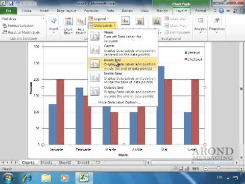
How to Change Excel Chart Data Labels to Custom Values? 05.05.2010 · Now, click on any data label. This will select “all” data labels. Now click once again. At this point excel will select only one data label. Go to Formula bar, press = and point to the cell where the data label for that chart data point is defined. Repeat the process for all other data labels, one after another. See the screencast. chandoo.org › wp › change-data-labels-in-chartsHow to Change Excel Chart Data Labels to Custom Values? Now, click on any data label. This will select "all" data labels. Now click once again. At this point excel will select only one data label. Go to Formula bar, press = and point to the cell where the data label for that chart data point is defined. Repeat the process for all other data labels, one after another. See the screencast. Points to note: How to add data labels from different column in an Excel chart? Reuse Anything: Add the most used or complex formulas, charts and anything else to your favorites, and quickly reuse them in the future. More than 20 text features: Extract Number from Text String; Extract or Remove Part of Texts; Convert Numbers and Currencies to English Words. Merge Tools: Multiple Workbooks and Sheets into One; Merge Multiple Cells/Rows/Columns … Adding rich data labels to charts in Excel 2013 | Microsoft 365 Blog Putting a data label into a shape can add another type of visual emphasis. To add a data label in a shape, select the data point of interest, then right-click it to pull up the context menu. Click Add Data Label, then click Add Data Callout . The result is that your data label will appear in a graphical callout.

How to add data labels in excel to graph or chart (Step-by-Step) To display extra data for a data series or data label, right-click it and select Format Data Labels. 2. Select the Values From Cells checked under Label Contains under Label Options. 3. Return to the spreadsheet and pick the range for which you want the cell values to show as data labels when the Data Label Range dialogue box displays. Chart: Display alternative values as Data Labels or Data Callouts Joined. Aug 11, 2017. Messages. 1. Aug 11, 2017. #1. Below is my excel chart. I would like to add a "data labels" or "data callouts". As you can see the line is displaying the data from Actual X and Y, but I want to display the DEV values on this line. How to I rotate data labels on a column chart so that they are ... To change the text direction, first of all, please double click on the data label and make sure the data are selected (with a box surrounded like following image). Then on your right panel, the Format Data Labels panel should be opened. Go to Text Options > Text Box > Text direction > Rotate Custom Chart Data Labels In Excel With Formulas - How To Excel At Excel Follow the steps below to create the custom data labels. Select the chart label you want to change. In the formula-bar hit = (equals), select the cell reference containing your chart label's data. In this case, the first label is in cell E2. Finally, repeat for all your chart laebls.

Example: Charts with Data Tools — XlsxWriter Documentation

Data Analysis in Excel (In Easy Steps) - Excel Easy 2 Filter: Filter your Excel data if you only want to display records that meet certain criteria. 3 Conditional Formatting: ... Use a line chart if you have text labels, dates or a few numeric labels on the horizontal axis. 26 Pie Chart: Pie charts are used to display the contribution of each value (slice) to a total (pie). Pie charts always use one data series. 27 Bar Chart: A bar chart is the ...

Format Number Options for Chart Data Labels in Excel 2011 for Mac

Add data labels and callouts to charts in Excel 365 - EasyTweaks.com Step #3: Format the data labels. Excel also gives you the option of formatting the data labels to suit your desired look if you don't like the default. To make changes to the data labels, right-click within the chart and select the "Format Labels" option.

Variable width column charts and histograms in Excel - Excel off the grid

Find, label and highlight a certain data point in Excel ... - Ablebits Select the Data Labels box and choose where to position the label. By default, Excel shows one numeric value for the label, y value in our case. To display both x and y values, right-click the label, click Format Data Labels…, select the X Value and Y value boxes, and set the Separator of your choosing: Label the data point by name

Using Excel 2010 - Add Data Labels - YouTube

Excel tutorial: How to use data labels Generally, the easiest way to show data labels to use the chart elements menu. When you check the box, you'll see data labels appear in the chart. If you have more than one data series, you can select a series first, then turn on data labels for that series only. You can even select a single bar, and show just one data label.

31 What Is Data Label In Excel - Labels Database 2020

› format-data-labels-in-excelFormat Data Labels in Excel- Instructions - TeachUcomp, Inc. Nov 14, 2019 · Then select the “Format Data Labels…” command from the pop-up menu that appears to format data labels in Excel. Using either method then displays the “Format Data Labels” task pane at the right side of the screen. Format Data Labels in Excel- Instructions: A picture of the “Format Data Labels” task pane in Excel.

Pie Chart - PK: An Excel Expert

Add a DATA LABEL to ONE POINT on a chart in Excel All the data points will be highlighted. Click again on the single point that you want to add a data label to. Right-click and select ' Add data label '. This is the key step! Right-click again on the data point itself (not the label) and select ' Format data label '. You can now configure the label as required — select the content of ...

November 2018

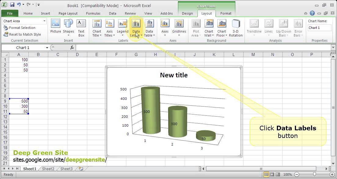
Adding Data Labels to Your Chart (Microsoft Excel) - ExcelTips (ribbon) To add data labels in Excel 2013 or Excel 2016, follow these steps: Activate the chart by clicking on it, if necessary. Make sure the Design tab of the ribbon is displayed. (This will appear when the chart is selected.) Click the Add Chart Element drop-down list. Select the Data Labels tool.

GANTT Procedure

Excel Chart Vertical Axis Text Labels • My Online Training Hub 14.04.2015 · Note: I didn’t have the original data for Juan's chart so I’ve recreated by eye and as a result the lines in my chart are slightly different to Juan’s, but the intention for this tutorial was to demonstrate how to display text labels in the vertical axis.

Tableau 201: How to Make a Highlight Table | Evolytics

Excel charts: how to move data labels to legend @Matt_Fischer-Daly . You can't do that, but you can show a data table below the chart instead of data labels: Click anywhere on the chart. On the Design tab of the ribbon (under Chart Tools), in the Chart Layouts group, click Add Chart Element > Data Table > With Legend Keys (or No Legend Keys if you prefer)

Excel Dashboards - Краткое руководство - CoderLessons.com

Format Data Labels in Excel- Instructions - TeachUcomp, Inc. 14.11.2019 · Format Data Labels in Excel: Instructions. To format data labels in Excel, choose the set of data labels to format. One way to do this is to click the “Format” tab within the “Chart Tools” contextual tab in the Ribbon. Then select the data labels to format from the “Current Selection” button group.

Working with Multiple Data Series in Excel | Pryor Learning Solutions

support.microsoft.com › en-us › officeEdit titles or data labels in a chart - support.microsoft.com To reposition all data labels for an entire data series, click a data label once to select the data series. To reposition a specific data label, click that data label twice to select it. This displays the Chart Tools , adding the Design , Layout , and Format tabs.

Custom data labels in a chart | Get Digital Help - Microsoft Excel resource

› charts › dynamic-chart-dataCreate Dynamic Chart Data Labels with Slicers - Excel Campus Feb 10, 2016 · Typically a chart will display data labels based on the underlying source data for the chart. In Excel 2013 a new feature called “Value from Cells” was introduced. This feature allows us to specify the a range that we want to use for the labels. Since our data labels will change between a currency ($) and percentage (%) formats, we need a ...

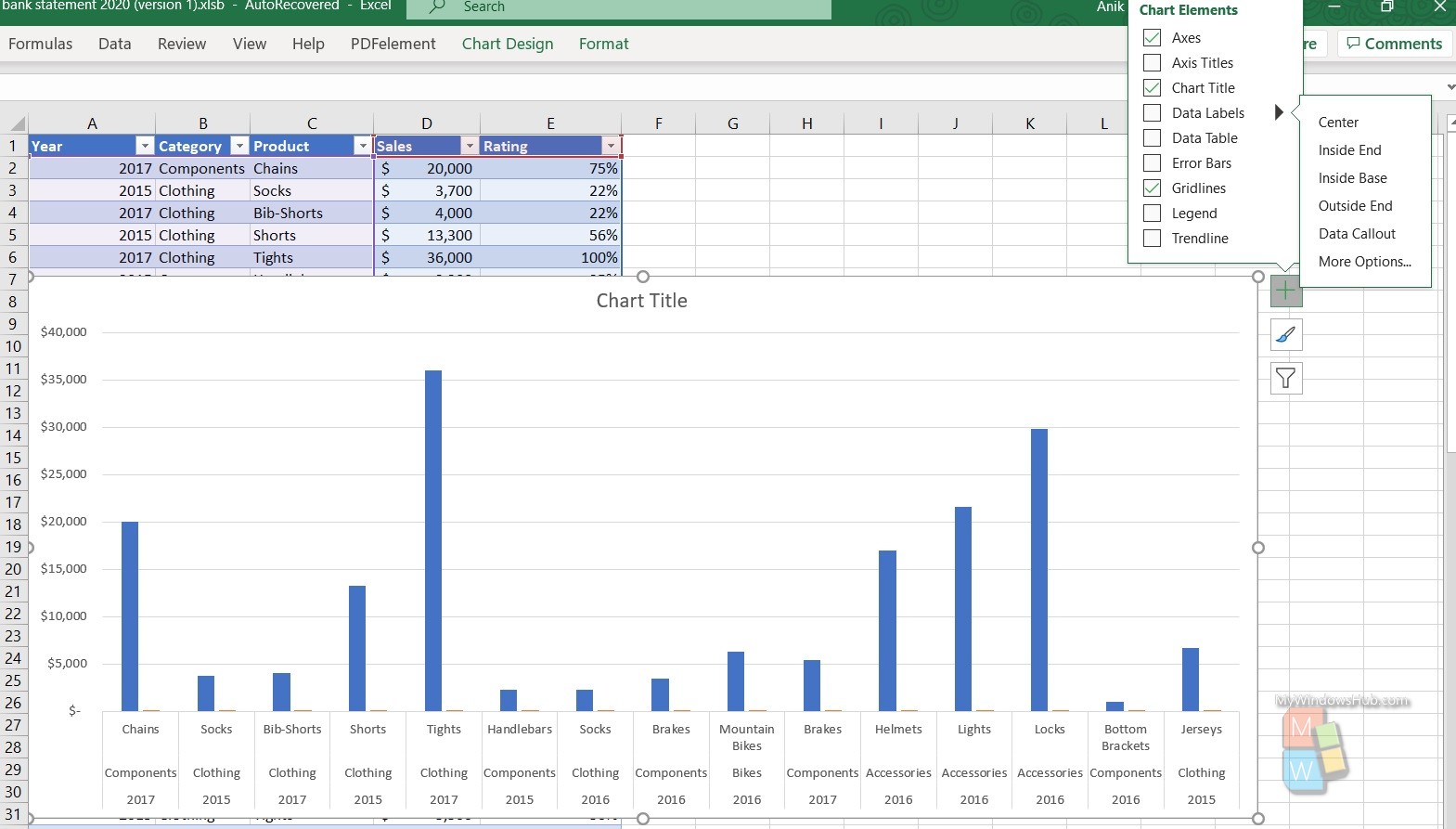
How To Show Or Hide Data Labels On MS Excel? | My Windows Hub

Edit titles or data labels in a chart - support.microsoft.com You can also place data labels in a standard position relative to their data markers. Depending on the chart type, you can choose from a variety of positioning options. On a chart, do one of the following: To reposition all data labels for an entire data series, click a data label once to select the data series.

MS Excel 2010 / How to remove data labels from the chart - YouTube

How to display text labels in the X-axis of scatter chart in Excel? Display text labels in X-axis of scatter chart. Actually, there is no way that can display text labels in the X-axis of scatter chart in Excel, but we can create a line chart and make it look like a scatter chart. 1. Select the data you use, and click Insert > Insert Line & Area Chart > Line with Markers to select a line chart. See screenshot:

WinForms Sankey Diagram - Data Visualization for .NET | DevExpress

How to Use Cell Values for Excel Chart Labels - How-To Geek Select the chart, choose the "Chart Elements" option, click the "Data Labels" arrow, and then "More Options." Uncheck the "Value" box and check the "Value From Cells" box. Select cells C2:C6 to use for the data label range and then click the "OK" button. The values from these cells are now used for the chart data labels.

How to Create Progress Charts (Bar and Circle) in Excel - Automate Excel

› documents › excelHow to add data labels from different column in an Excel chart? Click any data label to select all data labels, and then click the specified data label to select it only in the chart. 3. Go to the formula bar, type =, select the corresponding cell in the different column, and press the Enter key. See screenshot: 4. Repeat the above 2 - 3 steps to add data labels from the different column for other data points.

Format Data Labels in Excel- Instructions | Microsoft excel, Microsoft, Bar chart

Display Missing Dates in Excel PivotTables - My Online Training … 25.03.2014 · A regular PivotTable will only display the dates present in the source data. If you want to display the missing dates for March you need to take the following convoluted steps: Right-click one of the date row labels in the PivotTable > select Group > Days and Months: Next right-click one of the date row labels in the PivotTable > select Field Settings > Layout & Print …

Share :