42 excel pivot table conditional formatting row labels

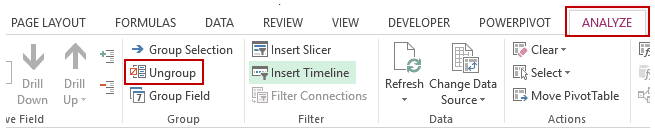
› excel-pivot-tables › the-pivotThe Pivot table tools ribbon in Excel These two tabs allow you to perform pivot table customization. This is the Pivot table ribbon in Excel. Create pivot table fields , charts and sets. Here is an important thing to wonder for the pivot table ribbon in excel is as soon as you switch the selected cell to non pivot table cell. The pivot table ribbon disappears. Re-Apply Pivot Table Conditional Formatting - yoursumbuddy This code identifies the first cell of the row label range and loops through each format condition in that cell and re-applies it to the range formed by the intersection of the row label range and the values range, i.e., the banded area in the first image above. This method relies on all the conditional formatting you want to re-apply being in ...

Excel Conditional Formatting in Pivot Table - EDUCBA Click on any cell in the pivot table > Go to the HOME tab > Click on Conditional Formatting option under Styles option > Click on Manage Rules option. It will open a Rules Manager dialog box. Click on the Edit Rule tab, as shown in the below screenshot. It will open the Editing Rule formatting window. Refer to the below screenshot.

Excel pivot table conditional formatting row labels

Pivot table conditional formatting based on row label işler Pivot table conditional formatting based on row label ile ilişkili işleri arayın ya da 21 milyondan fazla iş içeriğiyle dünyanın en büyük serbest çalışma pazarında işe alım yapın. Kaydolmak ve işlere teklif vermek ücretsizdir. Conditional Formatting in Pivot Table - WallStreetMojo To apply conditional formatting in the pivot table, first, we must select the column to format. In this example, select "Grand Total Column." Then, in the "Home" Tab in the "Styles" section, click on "Conditional Formatting." Consequently, a dialog box pops up. Then, we need to click on "New Rule." As a result, another dialog box will pop up. Apply Conditional Formatting | Excel Pivot Table Tutorial Go to Home Tab → Styles → Conditional Formatting → New Rule. From rule to, select the third option. And, from "select a rule" type select "Format only top or bottom" ranked values. In edit rule description, enter 1 in the input box and from the drop-down menu select "each Column Group". Apply formatting you want. Click OK.

Excel pivot table conditional formatting row labels. Pivot table conditional formatting - Exceljet Select any cell in the data you wish to format and then choose "New rule" from the conditional formatting menu on the Home tab of the ribbon. At the top of the window, you will see setting for which cells to apply conditional formatting to. For the example shown, we want: "All cells showing sum of "sales values" for name and "date" Travaux Emplois Pivot table conditional formatting based on row label ... Chercher les emplois correspondant à Pivot table conditional formatting based on row label ou embaucher sur le plus grand marché de freelance au monde avec plus de 21 millions d'emplois. L'inscription et faire des offres sont gratuits. Pivot Table with Conditional Formatting - Microsoft Community Pivot Table with Conditional Formatting. Ok, Pivot Tables are good, Pivot Tables are our friends. Now I want to use conditional formatting with a pivot table. I have seen a lot of examples, but none showing me how to use a field in the field list in the formula of a conditional format. Perhaps this is not possible, so I moved the field into a ... Pivot Table Conditional Formatting - Contextures Excel Tips We'll adjust the formatting range, to fix that problem. Select any cell in the pivot table. On the Ribbon's Home tab, click Conditional Formatting, then click Manage Rules. In the list of rules, select the Data Bar rule, which applies to cells B3:B8. Click Edit Rule, to open the Edit Formatting Rule window.

› blog › insert-blank-rows-inHow to Insert a Blank Row in Excel Pivot Table - MyExcelOnline Jan 17, 2021 · STEP 1: Click any cell in the Pivot Table. STEP 2: Go to Design > Blank Rows. STEP 3: You will need to click on the Blank Rows button and select Insert Blank Line After Each Item. NB: For this to work you will need at least two Pivot Table Items in the Rows Labels. You then get the following Pivot Table report: Conditional Format Pivot Table Row | Chandoo.org Excel Forums - Become ... Excel Ninja Apr 3, 2013 #2 Select the entire row, and when you apply the conditional format, make the column reference absolute. So, say we want the entire row 2 to be formatted if cell in col B = 5. formula would be: =$B2=5 Conditional formatting for Pivot Tables in Excel 2016 - Ablebits The format I used was to select Conditional Formatting > Top 10 Items > set it to 1 item and select the default format. This format can be copied from one range to the next if desired or built up for each range individually. To copy the format, select one or more cells with that format and click Copy. Excel VBA: Conditional Format of Pivot Table based on Column Label myPivotSourceName = myPivotField.Name. Then rather than referencing the data field with the pivot field object, I referenced the DataRange with the string: myPivotTable.PivotFields (myPivotSourceName).DataRange.Select. Works perfectly and is completely portable for any pivottable on any sheet with any fields. excel vba.

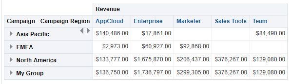
conditional formatting per row on pivot - Microsoft Tech Community I would like to format each row of a pivot table separately (as in the picture shown below), but I cannot paste the formatting. I've got many rows, and they could change (just like the columns) Is there a way to automate this, or I have to select row by row and apply the formatting? Even a "static" solution (a solution that doesn't follow the ... › blog › 101-excel-pivot-tables101 Excel Pivot Tables Examples | MyExcelOnline Jul 31, 2020 · Pivot Tables in Excel are one of the most powerful features within Microsoft Excel. An Excel Pivot Table allows you to analyze more than 1 million rows of data with just a few mouse clicks, show the results in an easy to read table, “pivot”/change the report layout with the ease of dragging fields around, highlight key information to management and include Charts & Slicers for your monthly ... trumpexcel.com › group-numbers-in-pivot-tableHow to Group Numbers in Pivot Table in Excel You May Also Like the Following Pivot Table Tutorials: How to Group Dates in Pivot Table in Excel. How to Create a Pivot Table in Excel. Preparing Source Data For Pivot Table. How to Refresh Pivot Table in Excel. Using Slicers in Excel Pivot Table – A Beginner’s Guide. How to Apply Conditional Formatting in a Pivot Table in Excel. How to Apply Conditional Formatting to Rows Based on ... - Excel Campus On the Home tab of the Ribbon, select the Conditional Formatting drop-down and click on Manage Rules…. That will bring up the Conditional Formatting Rules Manager window. Click on New Rule. This will open the New Formatting Rule window. Under Select a Rule Type, choose Use a formula to determine which cells to format.

Format Pivot Table Labels Based on Date Range Select all the dates in the Row Labels that you want to format. On the Ribbon, click the Home tab, and then in the Styles group, click Conditional Formatting. In the list of conditional formatting options, click Highlight Cells Rules, and then click A Date Occurring.

Conditional Formatting on Pivot Table row labels As per my knowledge, in this case it does not matter what is the source of pivot as after getting the data in pivot, it's the pivot where the conditional formatting need to be applied, please upload a sample. thanks. Regards, DILIPandey DILIPandey +91 9810929744 dilipandey@gmail.com Register To Reply

Using column label as formatting condition in excel pivot table I have pivot table in excel with sample data as attached. I now want to apply conditional formatting as red background where - data is between 10 to 25 AND - year is 2011 and 2012. =AND(C1="2011",OR(C2>10,C2<25)) how do i make cells example c2,c3,d2 red based on condition of year. Without Year condition it is working fine.

How to make row labels on same line in pivot table? Make row labels on same line with PivotTable Options You can also go to the PivotTable Options dialog box to set an option to finish this operation. 1. Click any one cell in the pivot table, and right click to choose PivotTable Options, see screenshot: 2.

Pivot table conditional formatting based on row label työt Etsi töitä, jotka liittyvät hakusanaan Pivot table conditional formatting based on row label tai palkkaa maailman suurimmalta makkinapaikalta, jossa on yli 21 miljoonaa työtä. Rekisteröityminen ja tarjoaminen on ilmaista.

Excel Pivot Table Conditional Formatting Row Labels Go making the conditional formatting select the color scale and do it based on commercial and choose diverging and the colors should give expected result. Here a glaze color or bar and been applied...

› pivot-tables › pivot-tableHow to Apply Conditional Formatting to Pivot Tables - Excel ... Dec 13, 2018 · How to Setup Conditional Formatting for Pivot Tables. Setting up conditional formatting for pivot tables is a little different than it is for regular cells/ranges. So in this post I explain how to apply conditional formatting for pivot tables. 1. Select a cell in the Values area. The first step is to select a cell in the Values area of the ...

› documents › excelHow to remove bold font of pivot table in Excel? - ExtendOffice The normal Bold feature can’t help us to un-bold the row labels in pivot table, but we can apply the powerful function – Conditional Formatting to solve this problem. Please do as follows: 1. Select the bold font row you want to un-bold in the pivot table, or you can press Ctrl key to select multiple bold font rows as your need. See screenshot:

Share :