39 how to add two data labels in excel pie chart

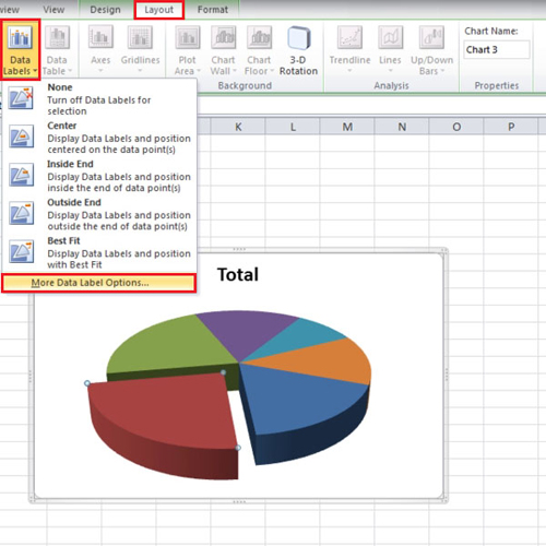
How To Make a Pie Chart in Excel (With Tips) | Indeed.com First, right-click on the pie chart and select "Add data labels" to insert the numerical value of each piece onto the pie chart. If you want your pieces to show category names, you can edit them by right-clicking any label and selecting "Format data labels," followed by "Label options." How do I create a dynamic chart in Excel? Here are the steps to insert a chart and use dynamic chart ranges: Go to the Insert tab. Click on 'Insert Line or Area Chart' and insert the 'Line with markers' chart. With the chart selected, go to the Design tab. Click on Select Data.

How to Create a Pie Chart in Google Sheets (With Example) Step 3: Customize the Pie Chart. To customize the pie chart, click anywhere on the chart. Then click the three vertical dots in the top right corner of the chart. Then click Edit chart: In the Chart editor panel that appears on the right side of the screen, click the Customize tab to see a variety of options for customizing the chart.

How to add two data labels in excel pie chart

How to Create Bar of Pie Chart in Excel - Computing.NET Step 1: Highlight the entire range. Step 2: Click on the Insert tab, Step 3: Navigate to the Chart grouping and click on the Insert Pie or Doughnut Chart icon. A drop-down box of Pie options is displayed. Step 4: Select the Bar of a Pie icon under the 2D pie category. This creates the combination as shown below. how to change legend name in excel pie chart Choose Add Date Labels>Add Data Callouts. To do this, right-click your graph or chart and click the "Select Data" option. Do not be lured by any of the other options, like exploded pie, or worst of all, a 3-D pie. Double-click the primary chart to open the Format Data Series window. This will replace the data labels in pie chart . excel pie chart from one column - perfectvisionksa.com Rotate 3-D charts in Excel: spin pie, column, line and bar charts. How to make a pie chart in Excel 1. We originally started with source data (on the Source Data sheet in the document) that consisted of two columns: item and a number. Object from the menu. You will learn about the various Excel charts types from column charts, bar charts, line ...

How to add two data labels in excel pie chart. Show data in a line, pie, or bar chart in canvas apps - Power Apps Add a pie chart. On the Insert tab, select Charts, and then select Pie Chart. Move the pie chart under the Import data button. In the pie-chart control, select the middle of the pie chart: Set the Items property of the pie chart to this expression: ProductRevenue.Revenue2014. The pie chart shows the revenue data from 2014. Display data point labels outside a pie chart in a paginated report ... Create a pie chart and display the data labels. Open the Properties pane. On the design surface, click on the pie itself to display the Category properties in the Properties pane. Expand the CustomAttributes node. A list of attributes for the pie chart is displayed. Set the PieLabelStyle property to Outside. Set the PieLineColor property to Black. Customize data labels in pandas pie chart - Stack Overflow I am trying to create a python pie chart from a dataframe with customized data labels. The dataframe that I am working off of contains percentages the correspond to each of the pie chart sections. I would like to display those percentages as data labels rather than the percent values of the totals of the whole. Excel does allow me to do that. Pie Chart in Excel - Inserting, Formatting, Filters, Data Labels To add Data Labels, Click on the + icon on the top right corner of the chart and mark the data label checkbox. You can also unmark the legends as we will add legend keys in the data labels. We can also format these data labels to show both percentage contribution and legend:- Right click on the Data Labels on the chart.

How to Make a Pie Chart in Microsoft Excel - groovyPost Go to the Insert tab and click the Pie Chart drop-down arrow. In Excel on the web, this is simply a button because there is currently only one pie chart design available. On Windows or Mac, select ... How to Create a Pie Chart from a Single Column [FREE Template ... Navigate to the Insert tab. Hit the " Insert Pie or Doughnut Chart " button. Under " 2-D Pie, " click " Pie. ". Once you do that, Excel will automatically plot a pie graph using your pivot table. Step 3. Clean up Your Pie Chart. Before calling it a day, let's remove the field buttons related to our pivot table to make the graph ... Pie Charts in Excel - F9 Finance Step 2: Select Range and Insert Chart. To insert a chart, you first need to highlight the data range. Make sure to pull in only the headers for product type or region as a pie chart can only work with one set of headers. Excel will automatically pull in the headers for you. Once you have highlighted the range, insert a standard pie chart ... Pie of Pie Chart in Excel - Inserting, Customizing, Formatting To add the data labels:- Select the chart and click on + icon at the top right corner of chart. Mark the check box containing data labels. Formatting Data Labels Consequently, this is going to insert default data labels on the chart.

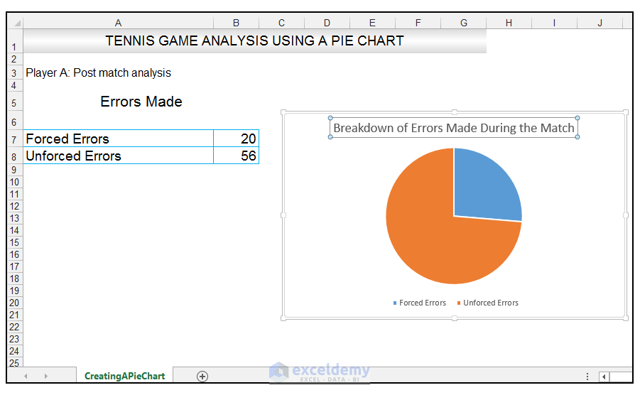
How to ☝️Create a Male/Female Pie Chart in Excel Click your pie chart to select it. 26. Open the Chart Design tab. 27. Click the "Add Chart Element" icon. 28. Choose "Data Labels." 29. Pick the best position or click "Data Callout" (this wraps data labels in a shape). Step 7. Add the Male/Female Icons Create Pie Chart In Excel - PieProNation.com Please do as follows to create a pie chart and show percentage in the pie slices. 1. Select the data you will create a pie chart based on, click Insert > I nsert Pie or Doughnut Chart > Pie. See screenshot: 2. Then a pie chart is created. Right click the pie chart and select Add Data Labels from the context menu. 3. how to change legend name in excel pie chart On the Insert tab of the ribbon, in the Charts group, click on the Insert Pie or Doughnut Chart button and in the opened menu, click on the first option among the 2-D Pie Charts. Step 6. Click anywhere on the chart. Click anywhere within your Excel chart, then click the Chart Elements button and check the Axis Titles box. About; . Assign specific colours to multiple Pivot Chart Data Series Hi All, hoping someone can help please! I have created Dashboards that contains approx. 40+ pivot chart across multiple tabs within a single excel worksheet. All the pivot table and data sources are contained in the same excel worksheet and the data sources are within a 'Dynamic' tables. Note: As this file is so large, complicated and confidential i cannot post an example, so apologies.

How to Make a Pie Chart in Excel & Add Rich Data Labels to The Chart!

How to Make a Pie Chart in Excel - WinBuzzer Right-click your graph and choose "Add Data Labels" Your data will automatically appear on the pie segments Customize them by right clicking the graph and pressing "Format Data Labels…" Tick what...

How to Make a Pie Chart in Excel & Add Rich Data Labels to The Chart!

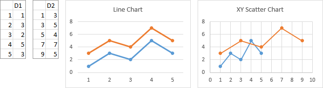
Plot Multiple Data Sets on the Same Chart in Excel Select the Chart -> Right Click on it -> Change Chart Type 2. The Chart Type dialog box opens. Now go to the " Combo " option and check the " Secondary Axis " box for the "Percentage of Students Enrolled" column. This will add the secondary axis in the original chart and will separate the two charts.

Excel Charting Dos and Don'ts - Peltier Tech Blog

How to Create Pie of Pie Chart in Excel? - GeeksforGeeks To add data in the secondary pie from the first pie, right Click on the second pie and choose Format Data Series. Here, the data series is split by percentage value and also customized the second plot by having values less than 15%. Now the pie of pie chart is formatted as follows:

How to Make a Pie Chart in Microsoft Excel 2010

how to group data in excel pie chart - perfectvisionksa.com Click add chart element and select data labels, and then select a location for the data label option. In the Charts group, click Pie. Click on the pie to select the whole pie. Excel can use the information already entered into a series of cells aligned in either a row or column of a spreadsheet to make a pie chart. In "By" enter 20.

Pie charts duel to their death: Create slope graphs as an alternative in Tableau in five steps

How To Create A Pie Chart In Excel - PieProNation.com With everything we need in place, its time to create a pie chart using the pivot table you just built. Select any cell in your pivot table . Navigate to the Insert tab. Hit the Insert Pie or Doughnut Chart button. Under 2-D Pie, click Pie. Once you do that, Excel will automatically plot a pie graph using your pivot table.

How to Make a Pie Chart in Excel & Add Rich Data Labels to The Chart!

How To Show Two Sets of Data on One Graph in Excel To do so, click and drag your mouse across all the data you want, including the names of the columns and rows. You can check that you selected the data by looking for the cells to be gray instead of white. 3. Click the "Insert" tab and then look at the "Recommended Charts" in the charts group

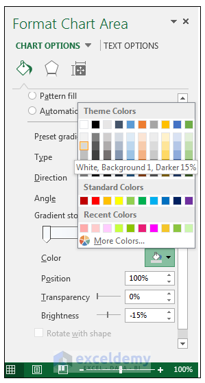
Change color of data label placed, using the 'best fit' option, outside a pie chart - Excel 2010 ...

excel pie chart from one column - perfectvisionksa.com Rotate 3-D charts in Excel: spin pie, column, line and bar charts. How to make a pie chart in Excel 1. We originally started with source data (on the Source Data sheet in the document) that consisted of two columns: item and a number. Object from the menu. You will learn about the various Excel charts types from column charts, bar charts, line ...

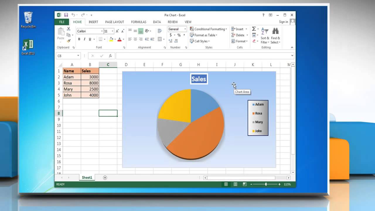
How to insert data labels in a Pie chart in Excel 2013 - YouTube

how to change legend name in excel pie chart Choose Add Date Labels>Add Data Callouts. To do this, right-click your graph or chart and click the "Select Data" option. Do not be lured by any of the other options, like exploded pie, or worst of all, a 3-D pie. Double-click the primary chart to open the Format Data Series window. This will replace the data labels in pie chart .