43 how to change axis labels in excel 2013
Excel 2013 - x Axis label alignment on a line chart (how ... Click here to reveal answer H Harry Flashman Active Member Joined May 1, 2011 Messages 356 Nov 14, 2016 #2 Sorry, I found it. Label alignment option maybe found under Size & Properties (the third icon on the top row of Format Axis options). You must log in or register to reply here. Similar threads S VBA for Chart Label , and axis sanket_sk Changing Axis Labels in PowerPoint 2013 for Windows Make sure you then deselect everything in the chart, and then carefully right-click on the value axis. Figure 2: Format Axis option selected for the value axis This step opens the Format Axis Task Pane, as shown in Figure 3, below. Make sure that the Axis Options button is selected as shown highlighted in red within Figure 3.
How to Change the X-Axis in Excel - Alphr Open the Excel file with the chart you want to adjust. Right-click the X-axis in the chart you want to change. That will allow you to edit the X-axis specifically. Then, click on Select Data. Next ...
How to change axis labels in excel 2013
How to group (two-level) axis labels in a chart in Excel? The Pivot Chart tool is so powerful that it can help you to create a chart with one kind of labels grouped by another kind of labels in a two-lever axis easily in Excel. You can do as follows: 1. Create a Pivot Chart with selecting the source data, and: (1) In Excel 2007 and 2010, clicking the PivotTable > PivotChart in the Tables group on the ... Adjusting the Angle of Axis Labels (Microsoft Excel) Right-click the axis labels whose angle you want to adjust. Excel displays a Context menu. Click the Format Axis option. Excel displays the Format Axis task pane at the right side of the screen. Click the Text Options link in the task pane. Excel changes the tools that appear just below the link. Click the Textbox tool. How to rotate axis labels in chart in Excel? If you are using Microsoft Excel 2013, you can rotate the axis labels with following steps: 1. Go to the chart and right click its axis labels you will rotate, and select the Format Axis from the context menu. 2.
How to change axis labels in excel 2013. Change axis labels in a chart in Office The chart uses text from your source data for axis labels. To change the label, you can change the text in the source data. If you don't want to change the text of the source data, you can create label text just for the chart you're working on. In addition to changing the text of labels, you can also change their appearance by adjusting formats. › excel › how-to-add-total-dataHow to Add Total Data Labels to the Excel Stacked Bar Chart Apr 03, 2013 · Step 4: Right click your new line chart and select “Add Data Labels” Step 5: Right click your new data labels and format them so that their label position is “Above”; also make the labels bold and increase the font size. Step 6: Right click the line, select “Format Data Series”; in the Line Color menu, select “No line” 3 Axis Graph Excel Method: Add a Third Y-Axis - EngineerExcel Add Data Labels To a Multiple Y-Axis Excel Chart. Axis labels were created by right-clicking on the series and selecting “Add ... (they would have corresponded directly to the secondary axis). However, in Excel 2013 and later, you can choose a range for the ... it’s simple to change the scaling factor and/or x-axis position of the third y ... Excel Chart Vertical Axis Text Labels • My Online Training Hub Click on the top horizontal axis and delete it. Hide the left hand vertical axis: right-click the axis (or double click if you have Excel 2010/13) > Format Axis > Axis Options: Set tick marks and axis labels to None. While you're there set the Minimum to 0, the Maximum to 5, and the Major unit to 1. This is to suit the minimum/maximum values ...
How to write range in excel - cosmoetica.it 'Write to Excel worksheet' write in A1 (row=1, column=1) the value A. Select an entire range of non-contiguous cells in a column. The second way to find the range is to use a combination of the SMALL and LARGE function. End(xlToLeft). Save the excel spreadsheet and after saving open the Excel spreadsheet. How to Add Total Data Labels to the Excel Stacked Bar Chart 3.4.2013 · I still can’t believe that Microsoft hasn’t fixed Office 2013 to allow you to just add a total to a stacked column chart. This solution works, but doesn’t look nearly as nice as a 3-D stacked column chart would. Also, some of the labels for the totals fall right on top the other column labels and therefore makes both of them unreadable. Reply support.microsoft.com › en-us › officeChange the scale of the vertical (value) axis in a chart To change the placement of the axis tick marks and labels, select any of the options in the Major tick mark type, Minor tick mark type, and Axis labels boxes. To change the point where you want the horizontal (category) axis to cross the vertical (value) axis, under Horizontal axis crosses , click Axis value , and then type the number you want ... How to Add Axis Labels in Excel 2013 - YouTube How to Add Axis Labels in Excel 2013For more tips and tricks, be sure to check out is a tutorial on how to add axis labels in E...
How to Change the Y Axis in Excel - Alphr To change the axis label's position, go to the "Labels" section. Click the dropdown next to "Label Position," then make your selection. Changing the Display of Axes in Excel How do I change the default chart axis colors of Excel 2013 One of these principles is that the axis color and labels should be muted and not be a stark black, to help the data points stand out better. If you are interested in learning good data visualisation, take a look at these books: With regards to your question: there is no Excel setting to change these colors by default. Creating a Third Axis In Excel - A Field Perspective on Engineering 19.4.2019 · For this example, I will set the axis up to plot the curves so they are not on top of each other, as illustrated above. Step 1 – Decide Which Data Series will use the “For Real” Excel Axes and Which will use the Third Axis. In the bigger picture, the first step in my process is to pick a scaling factor for your axes. Changing Axis Tick Marks (Microsoft Excel) Excel normally sets up the tick marks for you, but you can change the way they appear by following these steps if you are using Excel 2013 or a later version: Right-click on the axis whose tick marks you want to change. Excel displays a Context menu for the axis. Choose Format Axis from the Context menu.
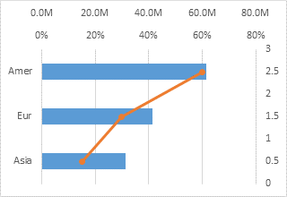
Bar-Line Chart with Secondary Axis or Two Panels - Peltier Tech Blog
Dynamically Label Excel Chart Series Lines - My Online Training … 26.9.2017 · To modify the axis so the Year and Month labels are nested; right-click the chart > Select Data > Edit the Horizontal (category) Axis Labels > change the ‘Axis label range’ to include column A. Step 2: Clever Formula. The Label Series Data contains a formula that only returns the value for the last row of data.

How to change chart axis labels' font color and size in Excel?
How to change chart axis labels' font color and size in Excel? (1) In Excel 2013's Format Axis pane, expand the Number group on the Axis Options tab, click the Category box and select Number from drop down list, and then click to select a red Negative number style in the Negative numbers box.
c# - Formatting Microsoft Chart Control X Axis labels for sub-categories to be like charts ...
Change axis labels in a chart - support.microsoft.com Right-click the category labels you want to change, and click Select Data. In the Horizontal (Category) Axis Labels box, click Edit. In the Axis label range box, enter the labels you want to use, separated by commas. For example, type Quarter 1,Quarter 2,Quarter 3,Quarter 4. Change the format of text and numbers in labels
Post a Comment for "43 how to change axis labels in excel 2013"